|
$ ised '#_{[10]}i{10*ran(1. 100000)}'
|
ten bins: roughly uniform distribution
|
|
9945 10059 9794 10076 10085 9984 9987 10146 10041 9883
|
|
|
$ ised '#_[10]iran(10. 100000)'
|
well, this is exactly the same
|
|
9897 10069 10115 10028 9874 10115 9929 9996 10051 9926
|
|
|
$ ised '#_[10]ran(10 100000)'
|
if fed integers, ran automatically generates integer numbers
|
|
9892 10135 9824 10131 9897 10084 9960 9987 10074 10016
|
|
|
$ ised '#_[10]i{10*sqtran(1. 100000)}'
|
if we take sqrt, distribution is linear
|
|
999 2975 4948 6966 9042 11162 13026 14959 16883 19040
|
|
|
$ ised '#__[0 0.1 1]{sqtran(1. 100000)}'
|
better way; first and last elements count outliers
|
|
0 1026 2863 4970 7058 8988 10899 12849 15052 16939 19356 0
|
|
|
$ ised '#_[2]ran(2 1000000)'
|
million coin flips
|
|
500520 499480
|
|
|
$ ised --F 'yes' --D 'no' '{0 0.}_ran2'
|
abuse of notation :)
|
|
no
|
or is it?
|
|
$ ised --F 'yes' --D 'no' '@0{ran2};{?$0}*0. {?{1-$0}}*0'
|
just to show how ? can be used to simulate if statement
|
|
yes
|
|
Explanation of last two examples: floats and integers use different print formats. So, if we yield float (0.) in case of 1 and int (0) in case of 0, we can
select which print routine will be used. We assigned two different strings to print formats.
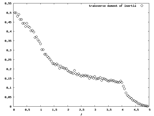
Here's more elaborate example. It calculates probability distribution of moment of inertia, if point mass is placed randomly into cylinder with height
"h" and unit radius. The script takes "N": number of samples, "h": height of cylinder and "binsize" width of bin for histogram.
This example illustrates how
|
ised> @0{0.05}
|
we choose step
|
|
0.05
|
|
|
ised> @1{[0 $0 pi]};
|
integration range
|
|
ised> @2{sin$1};
|
function values
|
|
ised> @3{$0*(0 $2 #$1)};
|
compute integral with starting point 0
|
|
ised> @4{{{$2<<-1}:-$2}/$0};
|
differentiate the same function
|
|
ised> --d "\t"
|
declare tab as separator
|
|
ised> --t '$1;$2;$3;$4'
|
output x, sin(x), its integral and derivative
|
|
0 0 0 0.999583
|
|
|
0.05 0.0499792 0 0.997085
|
|
|
0.1 0.0998334 0.00249896 0.992094
|
|
|
0.15 0.149438 0.00749063 0.984624
|
|
|
0.2 0.198669 0.0149625 0.974693
|
|
|
0.25 0.247404 0.024896 0.962325
|
|
|
0.3 0.29552 0.0372662 0.947552
|
|
|
...
|
|
|
2.8 0.334988 1.93344 -0.950203
|
|
|
2.85 0.287478 1.95019 -0.964574
|
|
|
2.9 0.239249 1.96457 -0.976534
|
|
|
2.95 0.190423 1.97653 -0.986053
|
|
|
3 0.14112 1.98605 -0.993107
|
|
|
3.05 0.0914646 1.99311 -0.99768
|
|
|
3.1 0.0415807 1.99768
|
|
Of course we can use any function or even load the values from a file, without modifying other steps.
|
ised> @1{0.237853 0.236133 0.0497423 0.145806 0.135682 0.231851 0.169376 0.0481285};
|
starting times (t1)
|
|
ised> @2{3.63055 3.87316 3.72171 3.87247 3.35336 3.56304 3.38296 3.34266};
|
finishing times (t2)
|
|
ised> 100/{$2:-$1}
|
velocities in meters per second
|
|
29.4751 27.495 27.2334 26.8337 31.0783 30.0193 31.1179 30.3533
|
|
|
ised> @+{$-1}/#$-1
|
compute average (using history value $-1)
|
|
29.2007
|
|
|
ised> avg$-2
|
easier way to get average (using the result two lines above with history $-2)
|
|
29.2007
|
|
|
ised> {$-1}*{3.6 1/0.44704}
|
convert to both km/h and mph
|
|
105.123 65.3201
|
|
There's no need to use memory, it's just more transparent for this tutorial. If the data set is small, we can just throw the numbers in:
|
ised> @1{2}@2{3}@3{-4}
|
prepare some values
|
|
2 3 -4
|
we will solve equation 2x^2+3x-4
|
|
ised> {-$2+pm*sqt{$2^2-4*$1*$3}}/{2*$1}
|
both solutions
|
|
0.850781 -2.35078
|
|
|
ised> $1*$-1^2:+$2*$-1:+$3*$-1^0
|
confirm results (note component-wise addition and use of last result $-1)
|
|
0 0
|
|
|
ised> pm
|
what pm actually is
|
|
1 -1
|
|
|
ised> pz${3 2 1}
|
builtin solver works just as well
|
|
0.850781 -2.35078
|
|
|
ised> px${3 2 1}$-1
|
builtin polynomial evaluator
|
|
-4.44089e-16 -0
|
polynomial evaluator may have some rounding issues
|
|
ised> @1{2}@2{3}@3{4}
|
now for equation with no real roots
|
|
2 3 4
|
|
|
ised> {-$2+pm*sqt{$2^2-4*$1*$3}}/{2*$1}
|
no change here: we just changed values in memory
|
|
nan nan
|
obviously no real roots
|
|
ised> pz${3 2 1}
|
builtin solver returns empty array
|
|
|
|
|
ised> @0{15}
|
choose number of terms
|
|
15
|
|
|
ised> @1{2.5}
|
choose some other value for x
|
|
2.5
|
|
|
ised> @+{$1^[$0]:/[$0]!} exp$1
|
exponential series and comparison with exact value
|
|
12.1825 12.1825
|
|
|
ised> (0 pm mp $0)
|
we find a way to generate factors for sine series
|
|
0 1 0 -1 0 1 0 -1 0 1 0 -1 0 1 0
|
|
|
ised> @+{(0 pm mp $0):*$1^[$0]:/[$0]!} sin$1
|
sine series and exact value
|
|
0.598473 0.598472
|
|
|
ised> @+{(1 -2 2 $0):*$1^O[$0]:/{O[$0]}!} sin$1
|
the same, but by selecting odd terms by operator O
|
|
0.598473 0.598472
|
|
|
ised> @+{(1 -2 2 $0):*$1^E[$0]:/{E[$0]}!} cos$1
|
cosine: the same, just select even terms
|
|
-0.801144 -0.801144
|
|
|
ised> (1 -2 2 $0)
|
just to see what we did there
|
|
1 -1 1 -1 1 -1 1 -1 1 -1 1 -1 1 -1 1
|
|
We can also generate sequences if we know the general term. For primes, we just remove all values that are products of some two numbers.
|
ised> @0{20}
|
how many terms
|
|
20
|
|
|
ised> @1 {0.5*{1+sqt5}}
|
precompute golden section
|
|
1.61803
|
|
|
ised> r{{$1^[1 $0]:-(-$1)^-[1 $0]}/sqt5}
|
Fibonacci sequence (note rounding to convert to integers)
|
|
1 1 2 3 5 8 13 21 34 55 89 144 233 377 610 987 1597 2584 4181 6765
|
|
|
ised> @+{[$0]^3} {@+[$0]}^2
|
interesting equality of sums
|
|
36100 36100
|
|
|
ised> @0{10}
|
now less terms
|
|
10
|
|
|
ised> $0!/{[0 $0]!:*~[0 $0]!}
|
binomial coefficients
|
|
1 10 45 120 210 252 210 120 45 10 1
|
|
|
ised> {1 1}**{1 1}**{1 1}**{1 1}
|
definition of binomial coefficients
|
|
1 4 6 4 1
|
|
|
ised> 4c[0 4]
|
built-in function for binomial coefficients
|
|
1 4 6 4 1
|
|
|
ised> @2[2 100];$2\{$2*$2}
|
primes up to 100
|
|
2 3 5 7 11 13 17 19 23 29 31 37 41 43 47 53 59 61 67 71 73 79 83 89 97
|
|
Recursively defined sequences cannot be evaluated directly because
|
ised> @1{: {x/2 3*x+1}_{x%2} :};
|
function that finds the next term
|
|
ised> @2{: @0{$0+1}*{} x :};
|
increments $0 silently and leaves x intact
|
|
ised> @3{: Q{103 -{x==1}} x :};
|
break if x==1, otherwise return to 0th function
|
|
ised> @0{1};
|
reset step counter
|
|
ised> ${1 2 3}::27
|
compute the sequence for 27
|
|
1
|
the iteration stops at 1
|
|
ised> $0
|
how many steps?
|
|
112
|
|
|
ised> @4{: @10{$10 x}*{} x:};
|
this function appends x to $10
|
|
ised> ${1 2 4 3}::27;
|
appending before loop test!
|
|
ised> $10
|
this contains the sequence now
|
|
82 41 124 62 31 ... 20 10 5 16 8 4 2 1
|
|
This shows that although the code is short, it is quite elaborate and requires care
to keep track of everything. The operator
|
ised> @2[2 50];$2\{$2*$2}
|
slow and dirty calculation
|
|
2 3 5 7 11 13 17 19 23 29 31 37 41 43 47
|
primes up to 50
|
|
ised> X[2 50]
|
built-in Miller-Rabin primality test
|
|
2 3 5 7 11 13 17 19 23 29 31 37 41 43 47
|
the same
|
|
ised> F@*X[2 50]
|
factorization retrieves the factors
|
|
2 3 5 7 11 13 17 19 23 29 31 37 41 43 47
|
|
|
ised> F10101
|
a composite number
|
|
3 7 13 37
|
prime factors
|
|
ised> ?{0==10101%[10101]}
|
[10101]} % divisors of above number
|
|
1 3 7 13 21 37 39 91 111 259 273 481 777 1443 3367
|
|
|
ised> phi{7 77 777 7777}
|
Euler Totient function
|
|
6 60 432 6000
|
|
|
ised> @1{3 12}/gcd$1
|
reducing a fraction
|
|
1 4
|
3/12 equals 1/4
|
|
ised> gcd{45 60 30} lcm{45 60 30}
|
works for multiple arguments
|
|
15 180
|
greatest common divisor and least common multiple
|
|
ised> F{123456789123456789}
|
large numbers are not a problem
|
|
3 3 7 11 13 19 3607 3803 52579
|
|
|
ised> max{pm**X[10000]}
|
max prime gap up to 10000
|
|
36
|
|
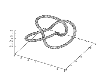
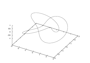 With a bit more effort, the knot can be visualized as a tube-like surface.
First and second derivative of the curve is first generated, then it is used
to generate normal and binormal and spaced by empty lines using a trick
involving switch --p. Then --t is used to convert each
line into a long column describing the circular (or any other) cross
section of the knot surface. Instead of piping one ised into another, --o
switch enables storage of intermediate files, so the entire procedure can be
done in a single script. Click on the image to see the ised script
that generated the data.
With a bit more effort, the knot can be visualized as a tube-like surface.
First and second derivative of the curve is first generated, then it is used
to generate normal and binormal and spaced by empty lines using a trick
involving switch --p. Then --t is used to convert each
line into a long column describing the circular (or any other) cross
section of the knot surface. Instead of piping one ised into another, --o
switch enables storage of intermediate files, so the entire procedure can be
done in a single script. Click on the image to see the ised script
that generated the data.